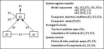
Figure 2: Illustration of component parameterisation for model generation


Figure 2 illustrates how the parameterisation process works. The diagram on the left gives a typical example of the relationships between the data structures involved, whilst the items on the right show where these come from and the division between automated and human responsibilities when using the method. Each component is designed to supply the definitions needed to satisfy a particular predicate ( e.g. to calculate biomass) and there may be numerous alternative components for any given predicate ( e.g. there are many standard ways to calculate biomass in a population dynamics model). Model construction is driven by the introduction of a ``top level'' predicate, P1 in the illustration, which is to be the main output of the model. The parameterisation system finds those components which can construct a definition for P1 and chooses which is appropriate by prompting the ecologist for the conditions associated with it - in the illustration conditions C1 and C2 have been satisfied (and instantiated by the ecologist) in order to select and instantiate component S1. The use of S1 introduces a need to define predicates P2 and P3, which are used in the definition of S1 but not defined directly within that component. These are defined by S2 and S3 respectively, with the ecologist confirming and instantiating condition C3 which is a common prerequisite for both components. The process terminates when we have components providing definitions for every predicate that we have introduced. In doing this most of the complexity of the components is hidden from the ecologist, who controls only the choice of top level predicate and the instantiation of conditions used in selecting components.

Figure 2: Illustration of component parameterisation for model generation
To demonstrate how this works for our example
(although it omits the details of the dialogue between ecologist and
model generator) we use the diagrammatic representation which we
introduced in Figure 2, extended to the example model.
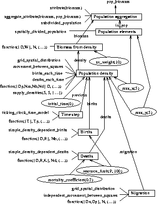
This is shown in Figure 3. Our top level predicate is
 and this is defined using Component 1, with the
ecologist having supplied the information that the attribute we are
concerned with is biomass (condition
  for
Component 1) and that this is aggregated into an attribute
describing the population biomass (condition
 for Component 1).
This introduces the need to define two new predicates: biomass and
 . We leave to the reader the task of following down through the
chain of parameterisations used in Figure 3 to define these
and the other predicates we introduced during model generation. Notice
that to save space we haven't shown all the details of the functions used
to instantiate conditions of the form
  , where
I is the set of input variables; O is the output variable; and
 is the arithmetic function relating inputs to outputs. In the
diagram we show all instances of
  as
as  to denote that
the actual instantiation has been omitted. You can reconstruct the
actual instantiation by comparing the appropriate component to the predicate
definition which it generates. For example, Component 3 is used
to define biomass given the conditions that the average weight is 10
(written as
  ) and that there is a function relating
variables
  to variable N. Although not shown on the diagram,
the arithmetic function is:
  , as we
can see by looking at the generated definition.

Figure 3: Map of component parameterisation for our example


