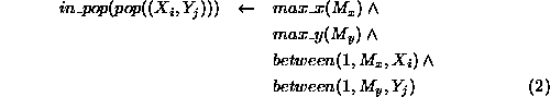
Our example is an animal population model based on a rectangular spatial grid. The grid has a fixed number of rows and columns and we know the initial population densities for each grid square. We will refer to the sub-populations in each square as population elements. Movement of animals can take place to neighbouring squares (those above, below, left or right of a given square) and this is observed as changes in the density of animals in the squares. The density of animals in a square may also change as a result of births and deaths. We are not interested in which individuals migrate, are born or die - our only interest is in the changes in the numbers of animals in each square (the population density) over time. In general, we are interested in the change of total biomass of the population over time, which is proportional to the total population density (assuming that we know the biomass of an ``average'' animal and that this multiplied by the density of animals gives a good approximation of the biomass in a unit area). The passage of time is represented using a simple ``ticking clock'', with the population densities at any given time being calculated from those of the previous ``tick''. The specification of our model is as follows, with expressions 1 to 13 defining the model and the expressions immediately following 13 defining its initialisation data.
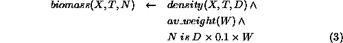
The biomass, N, of the population at time T is calculated by taking
the sum of the biomasses,  , of all the elements, X, of the
population.
, of all the elements, X, of the
population.
An element of the population, represented by the term
 exists for
  and
and
 , where
  and
and  are the maximum
numbered ``X'' and ``Y'' coordinate squares on the spatial grid.
are the maximum
numbered ``X'' and ``Y'' coordinate squares on the spatial grid.
The biomass, N, of any element, X, of the population at time, T, is calculated from that element's density, D multiplied by a fixed proportion of the average weight, W, of an animal in the population (the proportion being that of dry weight to total weight).
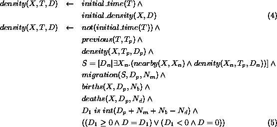
The density, D, of any element, X, of the population at time,
T, is either its initial density, if T is the initial time
(expression 4), or is
calculated from its density,  , at the previous time,
  ,
given the positive/negative effects of migration,
,
given the positive/negative effects of migration,  , from
nearby elements; the addition of births,
, from
nearby elements; the addition of births,  ; and subtraction of deaths,
 (expression 5).
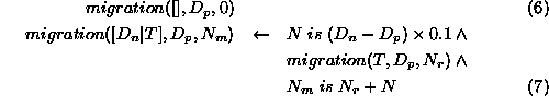
The number of animals migrating into a population element with
density  , given a list of the densities of its surrounding
elements, is obtained as follows. If the list of surrounding densities
is empty (expression 6) then migration is zero.
Otherwise, calculate the contribution to migration from the first element,
, given a list of the densities of its surrounding
elements, is obtained as follows. If the list of surrounding densities
is empty (expression 6) then migration is zero.
Otherwise, calculate the contribution to migration from the first element,
 , of the surrounding list as a proportion of the difference
between
, of the surrounding list as a proportion of the difference
between  and
and  (a positive value representing an influx into the element and a negative
value representing an exodus), and summing this with the total migration
to/from the rest of the list.
(a positive value representing an influx into the element and a negative
value representing an exodus), and summing this with the total migration
to/from the rest of the list.
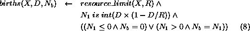
The number of animals born,  , in a population element, X,
with density, D, is a function of D and the resource limit, R, for
the population. This function will give low numbers of births at
low densities, increasing to a maximum at moderate densities, then
decreasing to zero at the resource limit.
, in a population element, X,
with density, D, is a function of D and the resource limit, R, for
the population. This function will give low numbers of births at
low densities, increasing to a maximum at moderate densities, then
decreasing to zero at the resource limit.
The number of deaths,  , in a population element, X,
with density, D, is a function of D; the resource limit, R, for
the population; and a mortality coefficient, K. This function will
give low numbers of deaths at low densities, increasing progressively as
density increases.
, in a population element, X,
with density, D, is a function of D; the resource limit, R, for
the population; and a mortality coefficient, K. This function will
give low numbers of deaths at low densities, increasing progressively as
density increases.
We are modelling time as a sequence of integer ``ticks'' so the
previous time point,  , from any time, T, is simply the previous
integer.
, from any time, T, is simply the previous
integer.
Given a population element of the form  , where X and
Y are the coordinates of the grid square for the element, we can find a
nearby element of the form
, where X and
Y are the coordinates of the grid square for the element, we can find a
nearby element of the form  , where
  is near to X
and
is near to X
and  is near to Y.
Grid square coordinate  is near to coordinate C, given that
the maximum coordinate value is
is near to coordinate C, given that
the maximum coordinate value is  if
if  is one above or below
the value of C without going outside the coordinate range
is one above or below
the value of C without going outside the coordinate range  .
.
The initial time is zero.

The average weight of animals is 10.

The coefficient for mortality is  .
.

The resource limit for all populations is 100.

The spatial grid has 5 rows and 5 columns.

The initial density, D, of population, X, is either stipulated using
 or it is not stipulated, in which case it is assumed to be
zero.
or it is not stipulated, in which case it is assumed to be
zero.

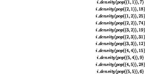
The stipulated initial densities for population elements at particular grid locations are as follows:
We can execute this specification directly using a Prolog interpreter. In particular, we can find out what will be the total biomass, N, of the population at any given time (say time 10) by satisfying the goal:

We can also find out the population density, D, for any element X at any time (say time 10) by satisfying the goal:

Figure 1 shows a plot of the biomass values generated by the model for times 0 to 10. These follow a curve upwards, levelling off to an asymptote, after which the total biomass fluctuates by only small amounts around a constant value. By looking at the changes of densities in grid squares over time - shown by the grids in Figure 1 - we can see why this happens. The first grid shows the initial distribution of animals, with two small clusters of higher density and the majority of the squares empty. By time 2 more of the squares are inhabited by migrations from the more heavily populated ones but the numbers of animals in each square are still low. By time 5 all of the squares are inhabited but the distribution of animals remains uneven. These differences have smoothed out by time 10 and migrations, deaths and births in each square are therefore approximately constant.