In this page we translate the information in Figure 2.6 into a more conventional logical notation, ready for further refinement. As in the translation of our operator diagram, the algorithm looks complex but can be automated. Our method for this is as follows:
 . Construct an expression:
  where
each
where
each  is a new variable restricted to type
  .
For example the top-level expression in Figure 2.6 is:
.
For example the top-level expression in Figure 2.6 is:  .
.
 on which it
depends (found by following backwards along the arrows on the diagram to its
data sources) and the type
on which it
depends (found by following backwards along the arrows on the diagram to its
data sources) and the type  of its result. Now construct a term
 where
each
where
each  is either a variable
  , if
, if  is the same type as
 , or, if not, is a new variable. Any new variables are
existentially quantified. For example the
, or, if not, is a new variable. Any new variables are
existentially quantified. For example the  function on
Figure 2.6 yields the expression:
function on
Figure 2.6 yields the expression:
 .
.
 , the left side of which comes from the first step and
where C is the conjunction of all the terms from the
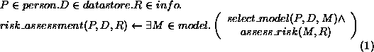
previous step. For our example, this gives us
expression 1 shown below.
, the left side of which comes from the first step and
where C is the conjunction of all the terms from the
previous step. For our example, this gives us
expression 1 shown below.
 on which it depends (by following backwards
along the arrows on the diagram to its data sources). Find the set of
data types
on which it depends (by following backwards
along the arrows on the diagram to its data sources). Find the set of
data types  which the function produces (by
following the arrows leading out of its oval). Construct an
expression
which the function produces (by
following the arrows leading out of its oval). Construct an
expression  where each
  is a new variable restricted to type
  .
All the variables
.
All the variables  are existentially quantified.
For example the
are existentially quantified.
For example the  function oval in Figure 2.6
yields expression 2 shown below.
function oval in Figure 2.6
yields expression 2 shown below.
We have a risk assessment for a person and some data source if there is some model which we can select for that person and data, and we can assess the loan risk based on that model.
For every person and data store we can select some model.