Mathematical Morphology is a tool for extracting image components that are useful for representation and description. The technique was originally developed by Matheron and Serra [3] at the Ecole des Mines in Paris. It is a set-theoretic method of image analysis providing a quantitative description of geometrical structures. (At the Ecole des Mines they were interested in analysing geological data and the structure of materials). Morphology can provide boundaries of objects, their skeletons, and their convex hulls. It is also useful for many pre- and post-processing techniques, especially in edge thinning and pruning.
Generally speaking most morphological operations are based on simple expanding and shrinking operations. The primary application of morphology occurs in binary images, though it is also used on grey level images. It can also be useful on range images. (A range image is one where grey levels represent the distance from the sensor to the objects in the scene rather than the intensity of light reflected from them).
The two basic morphological set transformations are erosion and dilation
These transformations involve the interaction between an image A (the object of interest) and a structuring set B, called the structuring element.
Typically the structuring element B is a circular disc in the plane, but it can be any shape. The image and structuring element sets need not be restricted to sets in the 2D plane, but could be defined in 1, 2, 3 (or higher) dimensions.
Let A and B be subsets of Z2. The translation of A by x is denoted Ax and is defined as
![]()
![]()
Dilation of the object A by the structuring element B is given by
![]()
The result is a new set made up of all points generated by obtaining the reflection of B about its origin and then shifting this relection by x.
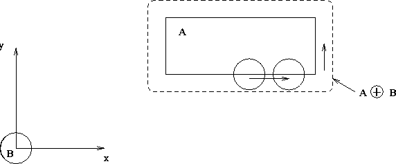
Consider the example where A is a rectangle and B is a disc
centred on the origin. (Note that if B is not centred on the origin we
will get a translation of the object as well.) Since B is symmetric,
![]() .
.
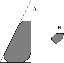
Erosion of the object A by a structuring element B is given by
![]()
![]()
![]()
![]()
![]()
Two very important transformations are opening and closing. Now intuitively, dilation expands an image object and erosion shrinks it. Opening generally smooths a contour in an image, breaking narrow isthmuses and eliminating thin protrusions. Closing tends to narrow smooth sections of contours, fusing narrow breaks and long thin gulfs, eliminating small holes, and filling gaps in contours.
The opening of A by B, denoted by ![]() , is given by the erosion
by B, followed by the dilation by B, that is
, is given by the erosion
by B, followed by the dilation by B, that is
![]()
 |
Opening is like `rounding from the inside': the opening of A by B is obtained by taking the union of all translates of B that fit inside A. Parts of A that are smaller than B are removed. Thus
![]()
Closing is the dual operation of opening and is denoted by ![]() .
It is produced by the
dilation of A by B, followed by the erosion by B:
.
It is produced by the
dilation of A by B, followed by the erosion by B:
![]()
Just as with dilation and erosion, opening and closing are dual operations. That is
![]()
The morphological filter ![]() can be used to eliminate
`salt and pepper' noise. Salt and pepper noise is random, uniformly distributed
small noisy elements often found corrupting real images. It will appear as
black dots or small blobs on a white background, and white dots or small
blobs on the black object. The background noise is eliminated at the erosion
stage, under the assumption that all noise components are physically
smaller than the structuring element B. Erosion on its own
will increase the size of the noise components on the object. However,
these are eliminated at the closing operation.
can be used to eliminate
`salt and pepper' noise. Salt and pepper noise is random, uniformly distributed
small noisy elements often found corrupting real images. It will appear as
black dots or small blobs on a white background, and white dots or small
blobs on the black object. The background noise is eliminated at the erosion
stage, under the assumption that all noise components are physically
smaller than the structuring element B. Erosion on its own
will increase the size of the noise components on the object. However,
these are eliminated at the closing operation.
The important thing to note is that morphological operations preserve the main geometric structures of the object. Only features `smaller than' the structuring element are affected by transformations. All other features at `larger scales' are not degraded. (This is not the case with linear transformations, such as convolution).
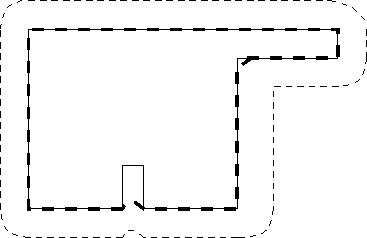
The boundary of a set A, denoted ![]() , can be
obtained by first eroding A with B, where B is a suitable
structuring element, and then performing the set difference between
A and its erosion. That is
, can be
obtained by first eroding A with B, where B is a suitable
structuring element, and then performing the set difference between
A and its erosion. That is
![]()
Region filling can be accomplished iteratively using dilations, complementation, and intersections. Suppose we have an image A containing a subset whose elements are 8-connected boundary points of a region. Beginning with a point p inside the boundary, the objective is to fill the entire region with 1s.
Since, by assumption, all non-boundary points are labeled 0, we begin by assigning 1 to p, and then construct
![]()
Likewise, connected components can also be extracted using morphological operations. If Y represents a connected component in an image A and a point p in Y is known, then the following iterative expression yields all the elements of Y:
![]()
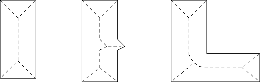
An important step in representing the structural shape of a planar region is to reduce it to a graph. This is very commonly used in robot path planning. This reduction is most commonly achieved by reducing the region to its skeleton.
The skeleton of a region is defined by the medial axis transformation (MAT). The MAT of a region R with border B is defined as follows: for each point p in R, we find its closest neighbour in B. If p has more than one such closest neighbour, then p belongs to the medial axis (or skeleton) of R. Of course, closest depends on the metric used. Figure 9 shows some examples with the usual Euclidean metric.
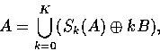
Direct implementation of the MAT is computationally prohibitive. However, the skeleton of a set can be expressed in terms of erosions and openings. Thus, it can be shown that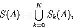
![\begin{displaymath}
S_k(A) = \bigcup_{k=0}^K \{(A \ominus kB) - [(A \ominus kB) \circ B], \end{displaymath}](img41.gif)
Thus A can be reconstructed from its skeleton subsets Sk(A) using the equation