The Fourier Transform is an
important image processing tool which is used to decompose an image
into its sine and cosine components. The output of the transformation
represents the image in the Fourier or frequency
domain, while the input image is the spatial domain
equivalent. In the Fourier domain image, each point represents a
particular frequency contained in the spatial domain image.
The Fourier Transform is used in a wide range of applications, such as image analysis, image filtering, image reconstruction and image compression.
As we are only concerned with digital images, we will restrict this discussion to the Discrete Fourier Transform (DFT).
The DFT is the sampled Fourier Transform and therefore does not contain all frequencies forming an image, but only a set of samples which is large enough to fully describe the spatial domain image. The number of frequencies corresponds to the number of pixels in the spatial domain image, i.e. the image in the spatial and Fourier domain are of the same size.
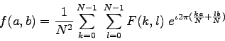
For a square image of size N×N, the two-dimensional DFT is given by:
where f(a,b) is the image in the spatial domain and the exponential term is the basis function corresponding to each point F(k,l) in the Fourier space. The equation can be interpreted as: the value of each point F(k,l) is obtained by multiplying the spatial image with the corresponding base function and summing the result.
The basis functions are sine and cosine waves with increasing frequencies, i.e. F(0,0) represents the DC-component of the image which corresponds to the average brightness and F(N-1,N-1) represents the highest frequency.
In a similar way, the Fourier image can be re-transformed to the
spatial domain. The inverse Fourier
transform is given by:
Note the  normalization term in the inverse transformation.
This normalization is sometimes applied to the forward transform instead of the
inverse transform, but it should not be used for both.$$
normalization term in the inverse transformation.
This normalization is sometimes applied to the forward transform instead of the
inverse transform, but it should not be used for both.$$
To obtain the result for the above equations, a double sum has to be calculated for each image point. However, because the Fourier Transform is separable, it can be written as
where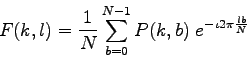
Using these two formulas, the spatial domain image is first transformed into an intermediate image using N one-dimensional Fourier Transforms. This intermediate image is then transformed into the final image, again using N one-dimensional Fourier Transforms. Expressing the two-dimensional Fourier Transform in terms of a series of 2N one-dimensional transforms decreases the number of required computations.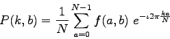
Even with these computational
savings, the ordinary one-dimensional DFT has  complexity. This can be reduced to
  if
we employ the Fast Fourier Transform (FFT) to compute the one-dimensional
DFTs. This is a significant improvement, in particular for
large images. There are various forms of the FFT and most of them
restrict the size of the input image that may be transformed, often to
if
we employ the Fast Fourier Transform (FFT) to compute the one-dimensional
DFTs. This is a significant improvement, in particular for
large images. There are various forms of the FFT and most of them
restrict the size of the input image that may be transformed, often to
 where n is an integer. The mathematical
details are well described in the literature.
where n is an integer. The mathematical
details are well described in the literature.
The Fourier Transform produces a complex number valued output image which can be displayed with two images, either with the real and imaginary part or with magnitude and phase. In image processing, often only the magnitude of the Fourier Transform is displayed, as it contains most of the information of the geometric structure of the spatial domain image. However, if we want to re-transform the Fourier image into the correct spatial domain after some processing in the frequency domain, we must make sure to preserve both magnitude and phase of the Fourier image.
The Fourier domain image has a much greater range than the image in the spatial domain. Hence, to be sufficiently accurate, its values are usually calculated and stored in float values.
The Fourier Transform is used if we want to access the geometric characteristics of a spatial domain image. Because the image in the Fourier domain is decomposed into its sinusoidal components, it is easy to examine or process certain frequencies of the image, thus influencing the geometric structure in the spatial domain.
In most implementations the Fourier image is shifted in such a way that the DC-value (i.e. the image mean) F(0,0) is displayed in the center of the image. The further away from the center an image point is, the higher is its corresponding frequency.
We start off by applying the Fourier Transform of
The magnitude calculated from the complex result is shown in
We can see that the DC-value is by far the largest component of the image. However, the dynamic range of the Fourier coefficients (i.e. the intensity values in the Fourier image) is too large to be displayed on the screen, therefore all other values appear as black. If we apply a logarithmic transformation to the image we obtain
The result shows that the image contains components of all frequencies, but that their magnitude gets smaller for higher frequencies. Hence, low frequencies contain more image information than the higher ones. The transform image also tells us that there are two dominating directions in the Fourier image, one passing vertically and one horizontally through the center. These originate from the regular patterns in the background of the original image.
The phase of the Fourier transform of the same image is shown in
The value of each point determines the phase of the corresponding frequency. As in the magnitude image, we can identify the vertical and horizontal lines corresponding to the patterns in the original image. The phase image does not yield much new information about the structure of the spatial domain image; therefore, in the following examples, we will restrict ourselves to displaying only the magnitude of the Fourier Transform.
Before we leave the phase image entirely, however, note that if we apply the inverse Fourier Transform to the above magnitude image while ignoring the phase (and then histogram equalize the output) we obtain
Although this image contains the same frequencies (and amount of frequencies) as the original input image, it is corrupted beyond recognition. This shows that the phase information is crucial to reconstruct the correct image in the spatial domain.
We will now experiment with some simple images to better understand the nature of the transform. The response of the Fourier Transform to periodic patterns in the spatial domain images can be seen very easily in the following artificial images.
The image
shows 2 pixel wide vertical stripes. The magnitude of the Fourier transform of this image is shown in
If we look carefully, we can see that it contains 3 main values: the DC-value and, since the Fourier image is symmetrical to its center, two points corresponding to the frequency of the stripes in the original image. Note that the two points lie on a horizontal line through the image center, because the image intensity in the spatial domain changes the most if we go along it horizontally.
The distance of the points to the center can be explained as follows: the maximum frequency which can be represented in the spatial domain are two pixel wide stripe pairs (one white, one black).
Hence, the two pixel wide stripes in the above image represent
Thus, the points in the Fourier image are halfway between the center and the edge of the image, i.e. the represented frequency is half of the maximum.
Further investigation of the Fourier image shows that the magnitude of
other frequencies in the image is less than
 of the DC-value, i.e. they don't make
any significant contribution to the image. The magnitudes of the two
minor points are each two-thirds of the DC-value.
of the DC-value, i.e. they don't make
any significant contribution to the image. The magnitudes of the two
minor points are each two-thirds of the DC-value.
Similar effects as in the above example can be seen when applying the Fourier Transform to
which consists of diagonal stripes. In
showing the magnitude of the Fourier Transform, we can see that, again, the main components of the transformed image are the DC-value and the two points corresponding to the frequency of the stripes. However, the logarithmic transform of the Fourier Transform,
shows that now the image contains many minor frequencies. The main reason is that a diagonal can only be approximated by the square pixels of the image, hence, additional frequencies are needed to compose the image. The logarithmic scaling makes it difficult to tell the influence of single frequencies in the original image. To find the most important frequencies we threshold the original Fourier magnitude image at level 13. The resulting Fourier image,
shows all
frequencies whose magnitude is at least 5% of the main peak. Compared
to the original Fourier image, several more points appear. They are
all on the same diagonal as the three main components, i.e. they all
originate from the periodic stripes. The represented frequencies are
all multiples of the basic frequency of the stripes in the spatial domain
image. This is because a rectangular signal, like the stripes, with
the frequency  is a composition of sine waves
with the frequencies
is a composition of sine waves
with the frequencies  ,
known as the harmonics of . All other
frequencies disappeared from the Fourier image, i.e. the magnitude of
each of them is less than 5% of the DC-value.
,
known as the harmonics of . All other
frequencies disappeared from the Fourier image, i.e. the magnitude of
each of them is less than 5% of the DC-value.
A Fourier-Transformed
image can be used for frequency filtering.
A simple example is illustrated with the above image. If we multiply
the (complex) Fourier image obtained above with an image containing a
circle (of r = 32 pixels), we can set all frequencies larger than
to zero as shown in the logarithmic
transformed image
By applying the inverse Fourier Transform we obtain
The resulting
image is a lowpass filtered version of the original spatial domain
image. Since all other frequencies have been suppressed, this result
is the sum of the constant DC-value and a sine-wave with the frequency
. Further examples can be seen in the
worksheet on frequency filtering.
A property of the Fourier Transform which is used, for example, for the removal of additive noise, is its distributivity over addition. We can illustrate this by adding the complex Fourier images of the two previous example images. To display the result and emphasize the main peaks, we threshold the magnitude of the complex image, as can be seen in
Applying the inverse Fourier Transform to the complex image yields
According to the distributivity law, this image is the same as the direct sum of the two original spatial domain images.
Finally, we present an example (i.e. text orientation finding) where the Fourier Transform is used to gain information about the geometric structure of the spatial domain image. Text recognition using image processing techniques is simplified if we can assume that the text lines are in a predefined direction. Here we show how the Fourier Transform can be used to find the initial orientation of the text and then a rotation can be applied to correct the error. We illustrate this technique using
a binary image of English text. The logarithm of the magnitude of its Fourier transform is
and
is
the thresholded magnitude of the Fourier image. We can see that the
main values lie on a vertical line, indicating that the text lines in
the input image are horizontal.
If we proceed in the same way with
which was rotated about 45°, we obtain
and
in the Fourier space. We can see that the line of the main peaks in the Fourier domain is rotated according to rotation of the input image. The second line in the logarithmic image (perpendicular to the main direction) originates from the black corners in the rotated image.
Although we managed to find a threshold which separates the main peaks from the background, we have a reasonable amount of noise in the Fourier image resulting from the irregular pattern of the letters. We could decrease these background values and therefore increase the difference to the main peaks if we were able to form solid blocks out of the text-lines. This could, for example, be done by using a morphological operator.
Another sinusoidal transform
(i.e. transform with sinusoidal base functions) related to the DFT is
the Discrete Cosine Transform (DCT). For an N×N image, the
DCT is given by
with
The
main advantages of the DCT are that it yields a real valued output
image and that it is a fast transform. A major use of the DCT is in
image compression --- i.e. trying to reduce the amount of data needed
to store an image. After performing a DCT it is possible to throw away
the coefficients that encode high frequency components that the human
eye is not very sensitive to. Thus the amount of data can be reduced,
without seriously affecting the way an image looks to the human eye.
You can interactively experiment with this operator by clicking here.
and
and add them using blend. Take the inverse Fourier Transform of the sum. Explain the result.
and compare its Fourier Transform before and after the operation.
and compare the Fourier Transforms with
with
and take the Fourier Transform. Compare the result with the multiplication of the two direct Fourier Transforms.
D. Ballard and C. Brown Computer Vision, Prentice-Hall, 1982, pp 24 - 30.
R. Gonzales, R. Woods Digital Image Processing, Addison-Wesley Publishing Company, 1992, pp 81 - 125.
B. Horn Robot Vision, MIT Press, 1986, Chaps 6, 7.
A. Jain Fundamentals of Digital Image Processing, Prentice-Hall, 1989, pp 15 - 20.
A. Marion An Introduction to Image Processing, Chapman and Hall, 1991, Chap. 9.
Specific information about this operator may be found here.
More general advice about the local HIPR installation is available in the Local Information introductory section.
©2003 R. Fisher, S. Perkins,
A. Walker and E. Wolfart.
![]()