Convolution is a simple mathematical operation which is fundamental to many common image processing operators. Convolution provides a way of `multiplying together' two arrays of numbers, generally of different sizes, but of the same dimensionality, to produce a third array of numbers of the same dimensionality. This can be used in image processing to implement operators whose output pixel values are simple linear combinations of certain input pixel values.
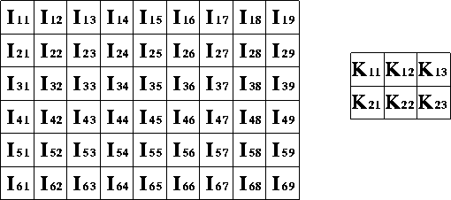
In an image processing context, one of the input arrays is normally just a graylevel image. The second array is usually much smaller, and is also two-dimensional (although it may be just a single pixel thick), and is known as the kernel. Figure 1 shows an example image and kernel that we will use to illustrate convolution.
Figure 1 An example small image (left) and kernel (right) to illustrate convolution. The labels within each grid square are used to identify each square.
The convolution is performed by sliding the kernel over the image, generally starting at the top left corner, so as to move the kernel through all the positions where the kernel fits entirely within the boundaries of the image. (Note that implementations differ in what they do at the edges of images, as explained below.) Each kernel position corresponds to a single output pixel, the value of which is calculated by multiplying together the kernel value and the underlying image pixel value for each of the cells in the kernel, and then adding all these numbers together.
So, in our example, the value of the bottom right pixel in the output image will be given by:
If the image has M rows and N columns, and the kernel has m rows and n columns, then the size of the output image will have M - m + 1 rows, and N - n + 1 columns.
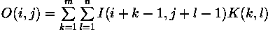
Mathematically we can write the convolution as:
where i runs from 1 to M - m + 1 and j runs from 1 to N - n + 1.
Note that many implementations of convolution produce a larger output image than this because they relax the constraint that the kernel can only be moved to positions where it fits entirely within the image. Instead, these implementations typically slide the kernel to all positions where just the top left corner of the kernel is within the image. Therefore the kernel `overlaps' the image on the bottom and right edges. One advantage of this approach is that the output image is the same size as the input image. Unfortunately, in order to calculate the output pixel values for the bottom and right edges of the image, it is necessary to invent input pixel values for places where the kernel extends off the end of the image. Typically pixel values of zero are chosen for regions outside the true image, but this can often distort the output image at these places. Therefore in general if you are using a convolution implementation that does this, it is better to clip the image to remove these spurious regions. Removing n - 1 pixels from the right hand side and m - 1 pixels from the bottom will fix things.
Convolution can be used to implement many different operators, particularly spatial filters and feature detectors. Examples include Gaussian smoothing and the Sobel edge detector.
You can interactively experiment with this operator by clicking here.
©2003 R. Fisher, S. Perkins,
A. Walker and E. Wolfart.
![]()